Examples
Test Cases
The sciform
test suite
contains hundreds of example formatting test cases which showcase the
many available formatting options.
Formatter
Here are a small selection of examples which demonstrate some of the available formatting options.
>>> from sciform import Formatter
>>> num = 12345.54321
>>> formatter = Formatter(exp_mode="scientific", round_mode="sig_fig", ndigits=4)
>>> print(formatter(num))
1.235e+04
>>> formatter = Formatter(
...     exp_mode="engineering",
...     round_mode="dec_place",
...     ndigits=10,
...     sign_mode=" ",
...     superscript=True,
... )
>>> print(formatter(num))
 12.3455432100×10³
>>> formatter = Formatter(
...     exp_mode="fixed_point",
...     upper_separator=" ",
...     decimal_separator=",",
...     lower_separator="_",
...     sign_mode="+",
... )
>>> print(formatter(num))
+12 345,543_21
>>> num = 0.076543
>>> formatter = Formatter(
...     exp_mode="scientific", exp_val=-3, exp_format="parts_per", add_ppth_form=True
... )
>>> print(formatter(num))
76.543 ppth
>>> formatter = Formatter(
...     exp_mode="scientific", exp_val=-2, exp_format="prefix", add_c_prefix=True
... )
>>> print(formatter(num))
7.6543 c
>>> formatter = Formatter(exp_mode="scientific", exp_val=-6, exp_format="prefix")
>>> print(formatter(num))
76543 μ
>>> formatter = Formatter(exp_mode="percent")
>>> print(formatter(num))
7.6543%
>>> num = 3141592.7
>>> unc = 1618
>>> formatter = Formatter()
>>> print(formatter(num, unc))
3141593 ± 1618
>>> formatter = Formatter(
...     exp_mode="engineering",
...     exp_format="prefix",
...     round_mode="pdg",
...     pm_whitespace=False,
... )
>>> print(formatter(num, unc))
(3.1416±0.0016) M
>>> num = 314159.27
>>> unc = 1618
>>> formatter = Formatter(
...     exp_mode="engineering_shifted", round_mode="pdg", paren_uncertainty=True
... )
>>> print(formatter(num, unc))
0.3142(16)e+06
Format Specification Mini Language
>>> from sciform import SciNum
>>> print(f"{SciNum(1234.432):0=+5.6f}")
+001234.432000
In the preceding example 0= indicates that left padding should be
done using '0' characters.
The + indicates that a sign symbol should always be displayed.
The 5 preceding the round mode symbol (.) indicates that the
number should be left padded to the 10+5 (ten-thousands)
decimal place.
The .6 indicates that the number will be rounded to six digits past
the decimal points.
The f indicates that the number will be displayed in fixed point
exponent mode.
>>> print(f"{SciNum(123, 0.123):#!2R()}")
0.12300(12)E+03
In the preceding example the # alternate flag combined with R
indicates that the number will be formatted in the shifted engineering
exponent mode with a capitalized exponent symbol 'E'.
!2 indicates that the number will be rounded so that the uncertainty
has two significant figures.
The () indicates that the value/uncertainty pair should be formatted
using the parentheses uncertainty format.
>>> print(f"{SciNum(123):ex-3p}")
123000 m
In the preceding example the e indicates that scientific notation
should be used.
The x-3 indicates that the exponent will be forced to equal -3.
Finally the p indicates that the SI prefix mode should be used.
>>> print(f"{SciNum(123): .-1f}")
 120
In this example the leading space indicates a leading space should be
included for non-negative numbers so that positive and negative numbers
have the same justification.
The .-1 indicates the number should be rounded to one
digit before the decimal point and the f indicates that fixed
point mode should be used.
>>> print(f"{SciNum(123.456, 0.123):Pf}")
123.46 ± 0.12
>>> print(f"{SciNum(123.456, 0.523):Pf}")
123.5 ± 0.5
>>> print(f"{SciNum(123.456, 0.973):Pf}")
123.5 ± 1.0
>>> print(f"{SciNum(123.456, 0.973):Af}")
123.456 ± 0.973
In these examples the "P" selects the "PDG" rounding rule and
"A" selects the "all" rounding rule.
SciNum, and Global Options
Here are a small selection of examples which demonstrate some of the
available string formatting options.
Note that many options are not available through the Format Specification Mini-Language, so
these options must be selected by configuring the global options.
Here this is done using the GlobalOptionsContext context
manager, but this could have been done using set_global_options()
instead.
>>> from sciform import SciNum, GlobalOptionsContext
>>> num = SciNum(12345.54321)
>>> print(f"{num:!4e}")
1.235e+04
>>> print(f"{num: .10r}")
 12.3455432100e+03
>>> with GlobalOptionsContext(
...     upper_separator=" ",
...     decimal_separator=",",
...     lower_separator="_",
... ):
...     print(f"{num:+}")
+12 345,543_21
>>> num = SciNum(0.076543)
>>> with GlobalOptionsContext(exp_format="parts_per", add_ppth_form=True):
...     print(f"{num:ex-3}")
...
76.543 ppth
>>> with GlobalOptionsContext(exp_format="prefix", add_c_prefix=True):
...     print(f"{num:ex-2}")
...
7.6543 c
>>> with GlobalOptionsContext(exp_mode="scientific", exp_val=-6, exp_format="prefix"):
...     print(f"{num:ex-6}")
...
76543 μ
>>> print(f"{num:%}")
7.6543%
>>> num_unc = SciNum(3141592.7, 1618)
>>> print(f"{num_unc}")
3141593 ± 1618
>>> with GlobalOptionsContext(round_mode="pdg", pm_whitespace=False):
...     print(f"{num_unc:rp}")
...
(3.1416±0.0016) M
>>> num_unc = SciNum(314159.27, 1618)
>>> with GlobalOptionsContext(round_mode="pdg"):
...     print(f"{num_unc:#r()}")
...
0.3142(16)e+06
Plotting and Tabulating Fit Data
We are given 3 data sets:
Data
{
    "data_0": {
        "x": [
            -0.0001,
            -7.777777777777778e-05,
            -5.555555555555556e-05,
            -3.3333333333333335e-05,
            -1.1111111111111112e-05,
            1.1111111111111112e-05,
            3.3333333333333335e-05,
            5.555555555555556e-05,
            7.777777777777778e-05,
            0.0001
        ],
        "y": [
            1000028705.1993496,
            1000032562.3072652,
            1000001896.3076739,
            1000015911.7068863,
            1000010552.1178038,
            1000024250.5937256,
            1000078382.654146,
            1000099609.1405739,
            1000156104.3810261,
            1000218228.6977944
        ],
        "y_err": [
            10074.736165669336,
            8935.559150444922,
            9783.419334631266,
            9603.772217328124,
            8958.492409007613,
            9691.25932834366,
            9465.18285498962,
            9252.428221037011,
            10506.00188280341,
            9674.67988710319
        ]
    },
    "data_1": {
        "x": [
            -0.0001,
            -7.777777777777778e-05,
            -5.555555555555556e-05,
            -3.3333333333333335e-05,
            -1.1111111111111112e-05,
            1.1111111111111112e-05,
            3.3333333333333335e-05,
            5.555555555555556e-05,
            7.777777777777778e-05,
            0.0001
        ],
        "y": [
            1000101738.923473,
            1000075626.403057,
            1000047095.4124904,
            1000035342.0517923,
            1000034627.8667482,
            1000024117.4097912,
            1000032427.2038687,
            1000058361.2708515,
            1000090132.8138337,
            1000137137.590938
        ],
        "y_err": [
            9546.933912908422,
            9865.10610577111,
            11233.801341794,
            8709.471433431938,
            9260.554239646424,
            11037.621922605267,
            11397.162303260564,
            10037.634586482105,
            10076.884695349665,
            9877.999777816845
        ]
    },
    "data_2": {
        "x": [
            -0.0001,
            -7.777777777777778e-05,
            -5.555555555555556e-05,
            -3.3333333333333335e-05,
            -1.1111111111111112e-05,
            1.1111111111111112e-05,
            3.3333333333333335e-05,
            5.555555555555556e-05,
            7.777777777777778e-05,
            0.0001
        ],
        "y": [
            1000162524.5101302,
            1000112400.2588283,
            1000095882.1735442,
            1000055167.7660033,
            1000026965.91884,
            1000019054.4158406,
            1000025166.114796,
            1000035728.0662737,
            1000075468.031305,
            1000105069.4047513
        ],
        "y_err": [
            10476.46500331082,
            10086.821923665966,
            9559.819918015002,
            10775.7594031851,
            11296.833796893989,
            10205.878907138671,
            10025.395431977211,
            10091.52840469254,
            11880.794221192386,
            10936.463066427263
        ]
    }
}
We want to perform quadratic fits to these data sets, visualize
the results, and print the best fit parameters including the uncertainty
reported by the fit routine.
For these tasks we will require the numpy, scipy,
matplotlib, and tabulate packages.
Without sciform
Without sciform we can perform the fit and plot the data and best
fit lines and print out a table of best fit parameters and
uncertainties:
Code
from __future__ import annotations

import json
from pathlib import Path
from typing import TYPE_CHECKING

import matplotlib.pyplot as plt
import numpy as np
from scipy.optimize import curve_fit
from tabulate import tabulate

if TYPE_CHECKING:
    from numpy.typing import NDArray


plt.style.use("dark_background")


def quadratic(x: NDArray, c: float, x0: float, y0: float) -> NDArray:
    return (c / 2) * (x - x0) ** 2 + y0


def main() -> None:
    data_path = Path("data", "fit_data.json")
    with data_path.open() as f:
        data_dict = json.load(f)

    color_list = ["red", "blue", "purple"]
    fit_results_list = []

    fig, ax = plt.subplots(1, 1)

    for idx, single_data_dict in enumerate(data_dict.values()):
        x = single_data_dict["x"]
        y = single_data_dict["y"]
        y_err = single_data_dict["y_err"]

        fit_results_dict = {}

        color = color_list[idx]
        ax.errorbar(x, y, y_err, marker="o", linestyle="none", color=color, label=color)

        # noinspection PyTupleAssignmentBalance
        popt, pcov = curve_fit(quadratic, x, y, sigma=y_err, p0=(2e13, 0, 1e9))

        model_x = np.linspace(min(x), max(x), 100)
        model_y = quadratic(model_x, *popt)
        ax.plot(model_x, model_y, color=color)

        fit_results_dict["color"] = color

        fit_results_dict["curvature"] = popt[0]
        fit_results_dict["curvature_err"] = np.sqrt(pcov[0, 0])

        fit_results_dict["x0"] = popt[1]
        fit_results_dict["x0_err"] = np.sqrt(pcov[1, 1])

        fit_results_dict["y0"] = popt[2]
        fit_results_dict["y0_err"] = np.sqrt(pcov[2, 2])

        fit_results_list.append(fit_results_dict)

    ax.grid(True)  # noqa: FBT003
    ax.legend()

    fig.savefig("outputs/fit_plot_no_sciform.png")
    plt.show()

    table_str = tabulate(
        fit_results_list,
        tablefmt="grid",
        headers="keys",
        floatfmt="#.2g",
    )
    table_path = Path("outputs", "fit_plot_no_sciform_table.txt")
    with table_path.open("w") as f:
        f.write(table_str)
    print(table_str)  # noqa: T201


if __name__ == "__main__":
    main()
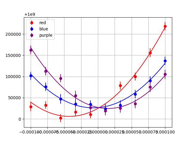
This produces the plot:
And the table:
+---------+-------------+-----------------+----------+----------+---------+----------+
| color   |   curvature |   curvature_err |       x0 |   x0_err |      y0 |   y0_err |
+=========+=============+=================+==========+==========+=========+==========+
| red     |     2.1e+13 |         1.9e+12 | -4.3e-05 |  4.8e-06 | 1.0e+09 |  4.6e+03 |
+---------+-------------+-----------------+----------+----------+---------+----------+
| blue    |     1.8e+13 |         1.0e+12 | -6.9e-06 |  1.6e-06 | 1.0e+09 |  2.9e+03 |
+---------+-------------+-----------------+----------+----------+---------+----------+
| purple  |     2.2e+13 |         1.7e+12 |  1.5e-05 |  2.5e-06 | 1.0e+09 |  4.4e+03 |
+---------+-------------+-----------------+----------+----------+---------+----------+
This plot and table suffer from a number of shortcomings which impede human readability.
In the table, the exponents for the values and uncertainties differ, making it hard to identify the significant digits of the value.
The number of digits displayed for the values is not correlated with the uncertainty for that value. For example, the
y0values are shown with precision to the 10+8 place, but the uncertainty indicates precision down to the 10+3 place.In the table, the exponents vary from one dataset to the next. It is hard to see these differences at a glance.
The tick labels on the plot are illegible because each value has so many digits.
Of course, even without sciform, it would be possible to make
manual adjustments to the plot and the table to improve these data
visualizations.
However, sciform will allow us to make the required changes in a
general and automated way.
With sciform
We can address these problems using sciform by:
Using prefix scientific notation to label the plot axes. This will greatly reduce the number of symbols needed for each tick value.
Using value/uncertainty formatting in the table to collapse the value and error column pairs into individual columns. This will make obvious the relative scale between the uncertainty and the value. Using
sciform, the significant digits displayed for the value will always match the precision of the uncertainty. We will use the parentheses uncertainty format.Using engineering notation for the value/uncertainty in the table. This will make the relative scale between different rows obvious.
To do this we import sciform and make some helper functions for
displaying the plot axes as described:
Code
from __future__ import annotations

import json
import re
from pathlib import Path
from typing import TYPE_CHECKING, Literal

import matplotlib.pyplot as plt
import numpy as np
from sciform import Formatter
from scipy.optimize import curve_fit
from tabulate import tabulate

if TYPE_CHECKING:
    from numpy.typing import NDArray


plt.style.use("dark_background")


def get_scale_and_offset_from_offset_str(
    ax: plt.Axes,
    axis: Literal["x", "y"],
) -> tuple[float, float]:
    """Get the scale and offset for an axis formatted in scientific mode."""
    plt.draw()
    if axis == "x":
        offset_text_obj = ax.xaxis.get_offset_text()
    elif axis == "y":
        offset_text_obj = ax.yaxis.get_offset_text()
    else:
        msg = f"axis must be 'x' or 'y', not '{axis}'."
        raise ValueError(msg)

    ax.ticklabel_format(axis=axis, style="sci")
    ax.get_figure().canvas.draw()  # Redraw canvas to update offset text
    offset_text = offset_text_obj.get_text()

    # Replace minus sign with hyphen minus sign
    offset_text = offset_text.replace("\u2212", "-")

    pattern = re.compile(r"^(?P<scale>1e[+-]?\d+)?(?P<offset>[+-]1e\d+)?$")
    match = re.match(pattern, offset_text)
    scale = float(match.group("scale") or 1)
    offset = float(match.group("offset") or 0)

    return scale, offset


def prefix_exp_ticks(
    ax: plt.Axes,
    axis: Literal["x", "y"],
    *,
    shifted: bool = False,
) -> None:
    """
    Use prefix notation for axis tick labels. Scale the tick labels by
    the multiplier that appears in the offset text and format the labels
    into SI prefix format. Format any remaining offset value in the
    offset text into SI prefix format as well.
    """
    if not shifted:
        exp_mode = "engineering"
    else:
        exp_mode = "engineering_shifted"
    # noinspection PyTypeChecker
    tick_formatter = Formatter(exp_mode=exp_mode, exp_format="prefix")
    # noinspection PyTypeChecker
    offset_formatter = Formatter(sign_mode="+", exp_mode=exp_mode, exp_format="prefix")

    ax.ticklabel_format(axis=axis, style="sci")

    if axis == "x":
        old_ticklabels = ax.get_xticklabels()
    elif axis == "y":
        old_ticklabels = ax.get_yticklabels()
    else:
        msg = f"axis must be 'x' or 'y', not '{axis}'."
        raise ValueError(msg)

    scale, offset = get_scale_and_offset_from_offset_str(ax, axis)

    new_tick_locations = []
    new_tick_labels = []
    for old_ticklabel in old_ticklabels:
        x, y = old_ticklabel.get_position()
        if axis == "x":
            new_tick_locations.append(x)
        else:
            new_tick_locations.append(y)

        # Replace minus sign with hyphen minus sign
        old_label_str = old_ticklabel.get_text().replace("\u2212", "-")
        val = float(old_label_str) * scale
        new_str = tick_formatter(val)
        new_tick_labels.append(new_str)

    if offset != 0:
        offset_str = offset_formatter(offset)
    else:
        offset_str = ""

    if axis == "x":
        ax.set_xticks(new_tick_locations, new_tick_labels)
        ax.text(x=1.01, y=0, s=offset_str, transform=ax.transAxes)
    else:
        ax.set_yticks(new_tick_locations, new_tick_labels)
        ax.text(x=0, y=1.01, s=offset_str, transform=ax.transAxes)


def quadratic(x: NDArray, c: float, x0: float, y0: float) -> NDArray:
    return (c / 2) * (x - x0) ** 2 + y0


def main() -> None:
    fit_results_formatter = Formatter(
        exp_mode="engineering",
        round_mode="sig_fig",
        paren_uncertainty=True,
        ndigits=2,
    )

    data_path = Path("data", "fit_data.json")
    with data_path.open() as f:
        data_dict = json.load(f)

    color_list = ["red", "blue", "purple"]
    fit_results_list = []

    fig, ax = plt.subplots(1, 1)

    for idx, single_data_dict in enumerate(data_dict.values()):
        x = single_data_dict["x"]
        y = single_data_dict["y"]
        y_err = single_data_dict["y_err"]

        fit_results_dict = {}

        color = color_list[idx]
        ax.errorbar(x, y, y_err, marker="o", linestyle="none", color=color, label=color)

        # noinspection PyTupleAssignmentBalance
        popt, pcov = curve_fit(quadratic, x, y, sigma=y_err, p0=(2e13, 0, 1e9))

        model_x = np.linspace(min(x), max(x), 100)
        model_y = quadratic(model_x, *popt)
        ax.plot(model_x, model_y, color=color)

        fit_results_dict["color"] = color
        fit_results_dict["curvature"] = fit_results_formatter(
            popt[0],
            np.sqrt(pcov[0, 0]),
        )
        fit_results_dict["x0"] = fit_results_formatter(popt[1], np.sqrt(pcov[1, 1]))
        fit_results_dict["y0"] = fit_results_formatter(popt[2], np.sqrt(pcov[2, 2]))

        fit_results_list.append(fit_results_dict)

    ax.grid(True)  # noqa: FBT003
    ax.legend()

    prefix_exp_ticks(ax, "x")
    prefix_exp_ticks(ax, "y", shifted=True)

    fig.savefig("outputs/fit_plot_with_sciform.png")
    plt.show()

    table_str = tabulate(fit_results_list, headers="keys", tablefmt="grid")
    table_path = Path("outputs", "fit_plot_with_sciform_table.txt")
    with table_path.open("w") as f:
        f.write(table_str)
    print(table_str)  # noqa: T201


if __name__ == "__main__":
    main()
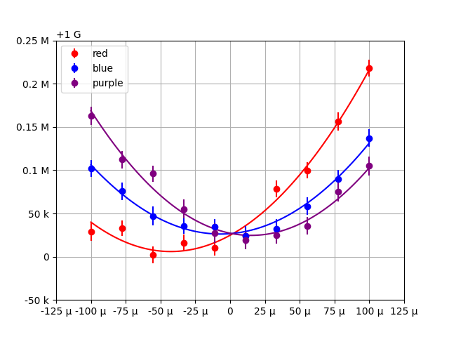
This produces the plot:
and the table:
+---------+---------------+----------------+-------------------+
| color   | curvature     | x0             | y0                |
+=========+===============+================+===================+
| red     | 20.7(1.9)e+12 | -42.7(4.8)e-06 | 1.0000060(46)e+09 |
+---------+---------------+----------------+-------------------+
| blue    | 18.4(1.0)e+12 | -6.9(1.6)e-06  | 1.0000262(29)e+09 |
+---------+---------------+----------------+-------------------+
| purple  | 21.7(1.7)e+12 | 15.1(2.5)e-06  | 1.0000246(44)e+09 |
+---------+---------------+----------------+-------------------+
We can see the plot and table are immediately much more legible. Less characters are needed to communicate the data in both visualizations. The relative scaling of parameters between datasets and the relative scaling between the value and uncertainty for each entry are immediately clear.
Mapping Over Collections
It may be convenient to apply sciform mapping to collections (sets,
lists, arrays, etc.) of numbers.
>>> from sciform import Formatter
>>>
>>> val_formatter = Formatter(
...     exp_mode="engineering",
...     exp_format="prefix",
...     round_mode="all",
...     paren_uncertainty=True,
... )
>>> val_err_formatter = Formatter(
...     exp_mode="engineering",
...     exp_format="prefix",
...     round_mode="pdg",
...     paren_uncertainty=True,
... )
>>> val_list = [1000, 2000, 3000]
>>> err_list = [200, 400, 600]
>>>
>>> val_str_list = list(map(val_formatter, val_list))
>>> print(val_str_list)
['1 k', '2 k', '3 k']
>>>
>>> val_err_str_list = list(map(val_err_formatter, val_list, err_list))
>>> print(val_err_str_list)
['1.00(20) k', '2.0(4) k', '3.0(6) k']
We may also want to map over higher dimensional numpy arrays. numpy.vectorize() makes this easy.
>>> import numpy as np
>>>
>>> vec_val_formatter = np.vectorize(val_formatter)
>>> vec_val_err_formatter = np.vectorize(val_err_formatter)
>>> arr = np.array([[1e6, 2e6, 3e6], [4e6, 5e6, 6e6], [7e6, 8e6, 9e6]])
>>>
>>> arr_err = np.array([[9e4, 8e4, 7e4], [6e4, 5e4, 4e4], [3e4, 2e4, 1e4]])
>>>
>>> print(vec_val_formatter(arr))
[['1 M' '2 M' '3 M']
 ['4 M' '5 M' '6 M']
 ['7 M' '8 M' '9 M']]
>>> print(vec_val_err_formatter(arr, arr_err))
[['1.00(9) M' '2.00(8) M' '3.00(7) M']
 ['4.00(6) M' '5.00(5) M' '6.00(4) M']
 ['7.000(30) M' '8.000(20) M' '9.000(10) M']]
Appending Units
The sciform SI prefix mode allows
exponent strings such as 'e+03' to be replaced with their SI
prefix counterparts such as 'k'.
In scientific applications numbers and numbers with uncertainty include
units such as 'g', 's', and 'Hz'.
The simple utility function below appends units to a sciform
output string in such a way that, if an SI prefix is present the unit
is appended to the prefix, otherwise there is a space between the unit
and the number.
>>> import re
>>> from sciform import FormattedNumber, SciNum
>>>
>>> def add_units(formatted_number: FormattedNumber, unit: str) -> FormattedNumber:
...     """Add units to a number string."""
...     if re.match(r"[a-zA-Z]", formatted_number[-1]):
...         num_with_units = f"{formatted_number}{unit}"
...     else:
...         num_with_units = f"{formatted_number} {unit}"
...     return FormattedNumber(
...         num_with_units,
...         formatted_number.value,
...         formatted_number.uncertainty,
...         formatted_number.populated_options,
...     )
>>>
>>> num_str = format(SciNum(123e6, 0.45e6), "rp()")
>>> print(num_str)
123.00(45) M
>>> print(add_units(num_str, "Hz"))
123.00(45) MHz
>>> num_str = format(SciNum(123, 0.45), "rp()")
>>> print(add_units(num_str, "Hz"))
123.00(45) Hz
>>> num_str = format(SciNum(123e6, 0.45e6), "e()")
>>> print(add_units(num_str, "Hz"))
1.2300(45)e+08 Hz
The utility function has been written to preserve the
FormattedNumber structure of the input so that the output
numbers with units can be still be e.g. converted to LaTeX:
>>> num_str = format(SciNum(123e6, 0.45e6), "rp()")
>>> print(add_units(num_str, "Hz").as_latex())
$123.00(45)\:\text{MHz}$
This utility function can be used for more complex units e.g.:
>>> num_str = format(SciNum(123e3, 0.45e3), "rp()")
>>> print(add_units(num_str, "m/s"))
123.00(45) km/s
however, you must remember that sciform, of course, only has
control over the single prefix out front.
If the user wants automated selection of multiple prefixes within a
compound unit such as 'cm/ms', then they will need to do logic to
determine the exact unit string or utilize a more sophisticated unit
framework.
At this point it would be recommended to, instead, directly calculate
the unit, rescale the numerical inputs to sciform formatting, and
append the entire unit without utilizing the sciform SI prefix
mode.
Interactions with the Decimal Module
Numbers passed into sciform are always converted into
Decimal instances during formatting.
Various options exposed by the
Decimal module
will (desirably or undesirably) modify sciform formatting
behavior.
>>> import decimal
>>> from sciform import SciNum
>>>
>>> # We calculate 1/9 in a high precision decimal context
>>> with decimal.localcontext() as ctx:
...     ctx.prec = 100
...     num = decimal.Decimal(1)/decimal.Decimal(9)
>>> # Formatted in the default decimal context
>>> print(format(SciNum(num), "Af"))
0.1111111111111111111111111111
>>>
>>> # Formatted in a low precision decimal context
>>> with decimal.localcontext() as ctx:
...     ctx.prec = 5
...     print(format(SciNum(num), "Af"))
0.11111
>>>
>>> # Formatted in a high precision decimal context
>>> with decimal.localcontext() as ctx:
...     ctx.prec = 50
...     print(format(SciNum(num), "Af"))
0.11111111111111111111111111111111111111111111111111
>>>
>>> # Formatted in a decimal context with a different rounding rule
>>> with decimal.localcontext() as ctx:
...     ctx.rounding = decimal.ROUND_CEILING
...     print(format(SciNum(num), "Af"))
0.1111111111111111111111111112
We see that the number of digits shown in the "all" round mode can
be modified using the decimal context precision.
We also see that the rounding mode can be adjusted away from the default
round-to-even rounding.
When working on high precision applications, recall that float
instances will always be converted to Decimal instances with 17
digits of precision or fewer.
So, if you desire higher precision you should use Decimal
rather than float inputs, otherwise you may observe undesirable
behavior.
See Note on Decimals and Floats.
Fallback Formatters
Sometimes values and value/uncertainty pairs with various properties may appear together in the same context. It may be inappropriate to use a single formatter for all of these inputs. For example
>>> from sciform import Formatter
>>> sform = Formatter(round_mode="pdg", paren_uncertainty=True)
>>> print(sform(123456, 0.0789))
123456.00(8)
>>> print(sform(123456, float("nan")))
120000(nan)
>>> print(sform(123456))
120000
In both the cases when the uncertainty was invalid for rounding and when the uncertainty wasn’t present the rounding got applied to the value directly. However, it may be inappropriate to apply PDG rounding, which is usually used for uncertainty, to the value. Instead, the user may want to retain more significant figures when rounding is applied to the value instead of the uncertainty. Users can resolve this by defining two formatters and a simple helper function to cover these cases.
>>> from math import isfinite
>>> from sciform import Formatter
>>>
>>> def generate_multi_formatter(
...     val_unc_formatter=None,
...     val_formatter=None
... ):
...     if val_unc_formatter is None:
...         val_unc_formatter = Formatter()
...     if val_formatter is None:
...         val_formatter = Formatter()
...     def multi_formatter(val, unc=None):
...         if unc is None or not isfinite(unc):
...             return val_formatter(val, unc)
...         else:
...             return val_unc_formatter(val, unc)
...     return multi_formatter
>>>
>>> multi_formatter = generate_multi_formatter(
...     val_unc_formatter = Formatter(
...         round_mode="pdg",
...         paren_uncertainty=True,
...     ),
...     val_formatter=Formatter(
...         round_mode="sig_fig",
...         ndigits=6,
...         paren_uncertainty=True,
...     ),
... )
>>>
>>> print(multi_formatter(123456, 0.0789))
123456.00(8)
>>> print(multi_formatter(123456, float("nan")))
123456(nan)
>>> print(multi_formatter(123456))
123456